Trees: Binary Trees, BST, and Balanced Trees
Imagine you need to store a million records and search through them efficiently. A sorted array gives you O(log n) search via binary search, but inserting a new element means shifting half the array on average. A linked list gives you O(1) insertion, but searching takes O(n). A tree gives you the best of both worlds: O(log n) search, insertion, and deletion (when balanced).
A tree is a data structure constructed with nodes, where each node has some value and may point to child nodes, which recursively form subtrees.
The first node in a tree is called the root. Nodes at the bottom of the tree that have no children are called leaf nodes (or just leaves).
The height of a tree is the length of its longest branch. Branches are paths between the root and its leaves.
The depth of a tree node is the distance from the tree’s root. It is also known as a node’s level in the tree.
A tree is essentially a graph that is connected and acyclic, has an explicit root node, and whose nodes all have a single parent (except the root node which has no parent). You can find out more about graphs in my graphs post. In most implementations, nodes do not have a pointer to their parent, but they can if desired.
There are many types of trees, like binary trees, heaps, AVL trees, and more.
Binary Tree
A binary tree is a tree whose elements have at most two children nodes. Here is the standard representation of a binary tree node in Java:
1
2
3
4
5
6
7
8
9
10
11
public class TreeNode {
    int value;
    TreeNode left;
    TreeNode right;

    public TreeNode(int value) {
        this.value = value;
        this.left = null;
        this.right = null;
    }
}
The structure of a binary tree is such that many of its operations have a logarithmic time complexity, making the binary tree an incredibly attractive and commonly used data structure. This logarithmic complexity holds for balanced binary trees: whenever we choose one child node, we effectively discard the other half of the remaining nodes. If the tree is unbalanced, operations may degrade to O(n) in the worst case.
Read more about logarithms in my logarithm post.
K-ary Tree
A k-ary tree is a tree whose nodes have up to k child nodes. A binary tree is a k-ary tree where k == 2.
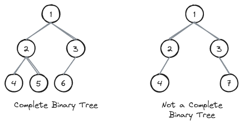
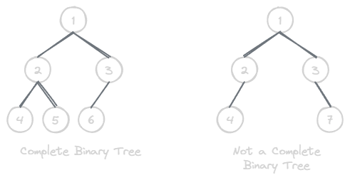
Complete Binary Tree
A complete binary tree is a binary tree that is almost perfect. All the levels are completely filled except possibly the lowest one, which is filled from the left. All the leaf elements must be as far left as possible.
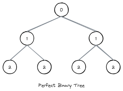
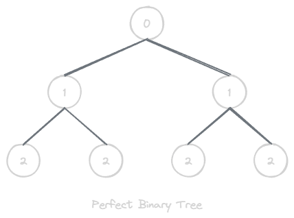
Perfect Binary Tree
A perfect binary tree is a binary tree whose interior nodes all have two child nodes and whose leaf nodes all have the same depth.
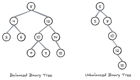
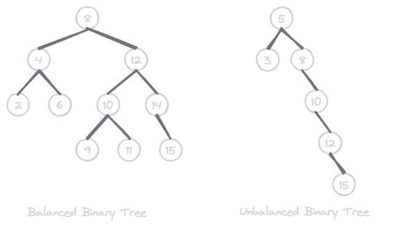
Balanced Binary Tree
A balanced binary tree is a binary tree whose nodes all have left and right subtrees whose heights differ by no more than 1.
A balanced binary tree is such that the logarithmic time complexity of its operations is maintained.
Why Balanced Trees Give O(log n) Performance
The key insight is that in a balanced binary tree, each level doubles the number of nodes. A tree with height h can hold at most 2^(h+1) - 1 nodes. Turning that around: if you have n nodes, the height is approximately log2(n).
Every operation (search, insert, delete) walks from the root down to at most one leaf, which means it visits at most h + 1 nodes. Since h is approximately log2(n), these operations run in O(log n) time.
When a tree becomes unbalanced, the height can grow up to n (a straight chain of nodes, like a linked list). Inserting a node at the bottom of such an imbalanced tree would clearly not be a logarithmic time operation, since it would involve traversing through most of the tree’s nodes.
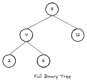
Full Binary Tree
A full binary tree is a binary tree whose nodes all have either two child nodes or zero child nodes.
Binary Search Tree (BST)
The most common tree variant is the Binary Search Tree. A BST is a binary tree where for every node, all values in its left subtree are less than the node’s value, and all values in its right subtree are greater. This ordering property allows for efficient searching: at each node, I can decide whether to go left or right, eliminating half the remaining nodes (in a balanced tree).
BST Search
Searching a BST exploits the ordering property. At each node, if the target value is smaller, go left. If it is larger, go right. If it matches, you have found it.
1
2
3
4
5
6
7
8
9
public TreeNode search(TreeNode root, int target) {
    if (root == null || root.value == target) {
        return root;
    }

    return (target < root.value)
            ? search(root.left, target)
            : search(root.right, target);
}
BST Insert
Insertion follows the same logic as search. Walk down the tree until you find a null spot where the new value belongs, then attach it there.
1
2
3
4
5
6
7
8
9
10
11
12
13
public TreeNode insert(TreeNode root, int value) {
    if (root == null) {
        return new TreeNode(value);
    }

    if (value < root.value) {
        root.left = insert(root.left, value);
    } else if (value > root.value) {
        root.right = insert(root.right, value);
    }
    // If value == root.value, it already exists (no duplicates)
    return root;
}
BST Delete
Deletion is the trickiest BST operation because it has three cases:
- Node is a leaf (no children): simply remove it.
- Node has one child: replace the node with its child.
- Node has two children: find the node’s inorder successor (the smallest value in its right subtree), copy that value into the node, then delete the successor.
1
2
3
4
5
6
7
8
9
10
11
12
13
14
15
16
17
18
19
20
21
22
23
24
25
26
27
28
29
30
31
public TreeNode delete(TreeNode root, int value) {
    if (root == null) {
        return null;
    }

    if (value < root.value) {
        root.left = delete(root.left, value);
    } else if (value > root.value) {
        root.right = delete(root.right, value);
    } else {
        // Found the node to delete
        if (root.left == null) {
            return root.right;
        }
        if (root.right == null) {
            return root.left;
        }
        // Node has two children: find inorder successor
        TreeNode successor = findMin(root.right);
        root.value = successor.value;
        root.right = delete(root.right, successor.value);
    }
    return root;
}

private TreeNode findMin(TreeNode node) {
    while (node.left != null) {
        node = node.left;
    }
    return node;
}
Self-Balancing Trees
Plain BSTs can become unbalanced over time. For example, inserting sorted data produces a degenerate tree that behaves like a linked list, where every operation degrades to O(n). Self-balancing trees solve this problem by automatically restructuring themselves during insertions and deletions through rotations.
A rotation is a local tree transformation that preserves the BST ordering property while changing the tree’s shape. The two fundamental rotations are:
- Left rotation: takes a node’s right child and promotes it to the node’s position, while the original node becomes the left child.
- Right rotation: the mirror of a left rotation.
Here is a right rotation in Java. The left rotation is symmetrical:
1
2
3
4
5
6
private TreeNode rotateRight(TreeNode node) {
    TreeNode newRoot = node.left;
    node.left = newRoot.right;
    newRoot.right = node;
    return newRoot;
}
Consider a simple case where we insert 3, 2, 1 into a BST. Without balancing, we get a left-leaning chain:
1
2
3
4
5
    3
   /
  2
 /
1
A right rotation on node 3 rebalances it:
1
2
3
  2
 / \
1   3
The BST property is preserved (1 < 2 < 3), but the height dropped from 3 to 2. This is the core mechanism that self-balancing trees use to maintain O(log n) height.
AVL Tree: the first self-balancing BST ever invented. It maintains the invariant that the heights of the left and right subtrees of every node differ by at most 1. After each insertion or deletion, rotations are performed to restore this balance. AVL trees provide strictly balanced structure, making lookups very fast, but insertions and deletions can be slightly more expensive due to the frequent rotations.
Red-Black Tree: a self-balancing BST where each node carries an extra bit of information: a color (red or black). A set of coloring rules ensures that the tree remains approximately balanced. No path from root to a leaf is more than twice as long as any other. Red-Black trees allow slightly less strict balancing than AVL trees, which means lookups can be marginally slower, but insertions and deletions are generally faster because fewer rotations are needed. Java’s
TreeMapandTreeSetuse Red-Black trees internally.
Tree Traversals
There are several standard ways to visit all nodes in a tree:
- Inorder (Left, Root, Right): visits nodes in ascending order for a BST.
- Preorder (Root, Left, Right): visits the root before its subtrees; useful for creating a copy of the tree.
- Postorder (Left, Right, Root): visits the root after its subtrees; useful for deleting a tree or evaluating expression trees.
- Level-order (BFS): visits nodes level by level from top to bottom.
Here is a recursive inorder traversal. For a BST, this prints all values in sorted order:
1
2
3
4
5
6
7
8
public void inorder(TreeNode root) {
    if (root == null) {
        return;
    }
    inorder(root.left);
    System.out.print(root.value + " ");
    inorder(root.right);
}
You can find detailed implementations of all traversal variants (including iterative approaches) in my Depth First Search in Java post.
Heaps
A heap is a specialized tree-based data structure that satisfies the heap property. In a max-heap, for every node, the value of the node is greater than or equal to the values of its children. In a min-heap, the value of the node is less than or equal to the values of its children.
Heaps are typically implemented as complete binary trees, which means they can be efficiently stored in an array without any pointers. For a node at index i:
- Left child is at index
2i + 1 - Right child is at index
2i + 2 - Parent is at index
(i - 1) / 2
This array representation is what makes heaps so memory-efficient compared to pointer-based tree structures.
Heap Operations
The two core operations are insertion and extraction:
- Insert: add the new element at the end (maintaining completeness), then “bubble up” by swapping with the parent as long as the heap property is violated. This runs in O(log n).
- Extract min/max: remove the root (the min or max element), move the last element to the root, then “bubble down” by swapping with the smaller (or larger) child until the heap property is restored. This also runs in O(log n).
1
2
3
4
5
6
7
8
9
10
11
12
13
14
15
16
17
18
19
20
21
22
23
24
25
26
27
28
29
30
31
32
33
34
35
36
37
38
39
40
41
42
43
44
45
46
47
48
49
50
51
52
53
54
55
56
57
public class MinHeap {
    private int[] heap;
    private int size;

    public MinHeap(int capacity) {
        this.heap = new int[capacity];
        this.size = 0;
    }

    public void insert(int value) {
        heap[size] = value;
        bubbleUp(size);
        size++;
    }

    public int extractMin() {
        int min = heap[0];
        size--;
        heap[0] = heap[size];
        bubbleDown(0);
        return min;
    }

    private void bubbleUp(int index) {
        while (index > 0) {
            int parent = (index - 1) / 2;
            if (heap[index] >= heap[parent]) {
                break;
            }
            swap(index, parent);
            index = parent;
        }
    }

    private void bubbleDown(int index) {
        while (2 * index + 1 < size) {
            int left = 2 * index + 1;
            int right = 2 * index + 2;
            int smallest = left;

            if (right < size && heap[right] < heap[left]) {
                smallest = right;
            }
            if (heap[index] <= heap[smallest]) {
                break;
            }
            swap(index, smallest);
            index = smallest;
        }
    }

    private void swap(int i, int j) {
        int temp = heap[i];
        heap[i] = heap[j];
        heap[j] = temp;
    }
}
When to Use Heaps
Heaps are the go-to data structure when you need efficient access to the minimum or maximum element. Common use cases include:
- Priority queues: Java’s
PriorityQueueis backed by a min-heap. - Finding the k-th largest/smallest element in a stream.
- Heap sort: an in-place O(n log n) sorting algorithm.
- Graph algorithms: Dijkstra’s shortest path and Prim’s minimum spanning tree both rely on heaps for their efficient implementations.
Complexity of Common Tree Operations
| Operation | BST (average) | BST (worst case) | Balanced BST (AVL / Red-Black) | Heap |
|---|---|---|---|---|
| Search | O(log n) | O(n) | O(log n) | O(n) |
| Insert | O(log n) | O(n) | O(log n) | O(log n) |
| Delete | O(log n) | O(n) | O(log n) | O(log n) |
| Find min/max | O(n) | O(n) | O(n) | O(1) |
The worst case for a plain BST occurs when the tree degenerates into a linear chain (e.g., inserting already-sorted data). Self-balancing trees guarantee O(log n) for search, insert, and delete regardless of the insertion order. Heaps trade general search efficiency for O(1) access to the min or max element.
When to Use Trees
Trees shine in situations that require ordered data with efficient insertion and deletion:
- Sorted dictionaries and sets: when you need keys in sorted order, a balanced BST (like Java’s
TreeMaporTreeSet) is ideal. - Range queries: finding all elements between two values is natural with BSTs.
- Priority-based processing: heaps (and by extension priority queues) are the right choice when you repeatedly need the smallest or largest element.
- Hierarchical data: file systems, organizational charts, and XML/HTML documents are naturally tree-shaped.
- Database indexes: B-trees and B+ trees (multi-way balanced trees) are the backbone of database indexing.
When Not to Use Trees
- Simple key-value lookups: if you do not need ordering, a hash table gives O(1) average-case lookups versus a tree’s O(log n).
- Small datasets: for small collections (say, under a few hundred elements), the overhead of maintaining tree structure is not worth it. A simple array or list will perform just as well in practice.
- Cache-sensitive workloads: trees have poor cache locality compared to arrays because nodes are scattered across memory. For performance-critical code with predictable access patterns, arrays or array-backed structures may be faster despite their worse theoretical complexity.
Related posts: Graphs, Depth First Search in Java, Logarithm, Data Structures Compendium