Specialized Storage Paradigms

In addition to widely known SQL and NoSQL databases, such as document or key-value stores, there are specialized storage paradigms that are well-suited for specific use cases.

Blob Storage

Blob storage is a common storage solution used in both small and large-scale systems. While not considered a database per se, it allows users to store and retrieve data based on a blob’s name. This is similar to a key-value store, but with different performance guarantees. Blob storage may be slower than key-value stores, but it can handle much larger values, such as megabytes or even gigabytes.

Common use cases for blob storage include storing large binaries, database snapshots, or static assets like images for websites. Blob storage infrastructure is complex to maintain on-premises and is typically provided by large companies like Google, Amazon, or Microsoft. In the context of system design interviews, you can assume the availability of GCS, S3, or Azure Blob Storage, which are blob storage services hosted by Google, Amazon, and Microsoft, respectively.

Working with Blob Storage

At its core, blob storage follows a key-value model: you address each object by a bucket (a logical container) and a key (the object’s name within that bucket). All operations go over HTTP, which makes the API simple but also means latency is higher than an in-process key-value store.

Here is a basic put/get example using the AWS SDK for Java (S3):

S3Client s3 = S3Client.builder()
        .region(Region.US_EAST_1)
        .build();

// Upload a file
s3.putObject(
        PutObjectRequest.builder()
                .bucket("my-app-assets")
                .key("images/profile/user-42.png")
                .contentType("image/png")
                .build(),
        Path.of("/tmp/user-42.png"));

// Download it back
s3.getObject(
        GetObjectRequest.builder()
                .bucket("my-app-assets")
                .key("images/profile/user-42.png")
                .build(),
        Path.of("/tmp/downloaded.png"));

Providers like S3, GCS, and Azure Blob Storage also support versioning, lifecycle rules (e.g. move to cold storage after 90 days), and multipart uploads for large files, but the fundamental interaction is always put and get by key.

Time Series Database

A Time Series Database (TSDB) is a specialized database optimized for storing and analyzing time-indexed data, data points occurring at specific moments in time. TSDBs are built around the assumption that data arrives in chronological order and is predominantly appended rather than updated in place, which allows them to use highly efficient compression and storage strategies.

Common TSDBs include InfluxDB, TimescaleDB (a PostgreSQL extension), Prometheus, and Graphite. Typical use cases extend well beyond basic monitoring:

• Infrastructure and application metrics: tracking CPU, memory, request latency, and error rates over time.
• IoT sensor data: ingesting millions of data points per second from connected devices.
• Financial data: storing tick-by-tick stock prices, trading volumes, and market indicators for time-based analysis.

TSDBs typically offer built-in support for downsampling, retention policies, and time-windowed aggregations, making them far more efficient for these workloads than a general-purpose relational database.

Writing and Querying Time Series Data

Most TSDBs use a compact write format optimized for append-heavy workloads. In InfluxDB, data is written using line protocol, where each line represents a single data point:

cpu_usage,host=server01,region=us-east value=72.5 1609459200000000000
cpu_usage,host=server01,region=us-east value=68.3 1609459260000000000
cpu_usage,host=server02,region=eu-west value=91.2 1609459200000000000

Each line follows the format measurement,tags fields timestamp. Tags are indexed metadata (like host and region) used for filtering, fields hold the actual measured values, and the timestamp is in nanosecond Unix time.

Querying is where TSDBs differentiate themselves from general-purpose databases. Here is a Flux query that computes average CPU usage in 5-minute windows for a specific host:

from(bucket: "metrics")
  |> range(start: -1h)
  |> filter(fn: (r) => r._measurement == "cpu_usage" and r.host == "server01")
  |> aggregateWindow(every: 5m, fn: mean)
  |> yield(name: "avg_cpu")

Time-windowed aggregation is a first-class concept in TSDBs. Queries like “average CPU per 5-minute bucket” or “99th percentile latency per hour” run efficiently because the storage engine is designed around time-ordered data and pre-built time indexes. Achieving the same in a relational database requires manual bucketing with DATE_TRUNC or similar functions and performs significantly worse at scale.

Graph Database

Graph databases store data using a graph data model, allowing data entries to have explicitly defined relationships, similar to nodes and edges in a graph. They can traverse millions of relationships in milliseconds because each node physically stores pointers to its adjacent nodes and edges (index-free adjacency). This means the cost of a traversal step is constant, regardless of the total size of the graph. By contrast, a relational database must execute JOIN operations for each hop, and each JOIN typically requires an index lookup whose cost grows logarithmically with table size. For multi-hop queries (e.g. “friends of friends of friends”), a graph database performs a fixed number of pointer dereferences per hop, while a relational database compounds JOIN costs at every level, making deep traversals orders of magnitude slower.

Graph databases are often preferred over relational databases when dealing with systems where data points naturally form a graph with multiple levels of relationships, such as social networks.

However, graph databases are not the right choice for every scenario. For simple relational data with well-defined schemas and straightforward join patterns, a traditional SQL database will typically outperform a graph database and be easier to maintain. Graph databases can also struggle with high-write, bulk-ingest workloads, as maintaining index structures for edges and nodes adds overhead compared to row-oriented or column-oriented stores.

Cypher

Cypher is a graph query language originally developed for the Neo4j graph database but has since been standardized for use with other graph databases, aiming to become the “SQL for graphs.” Cypher queries are generally simpler than their SQL counterparts because the syntax mirrors the shape of the graph you are traversing.

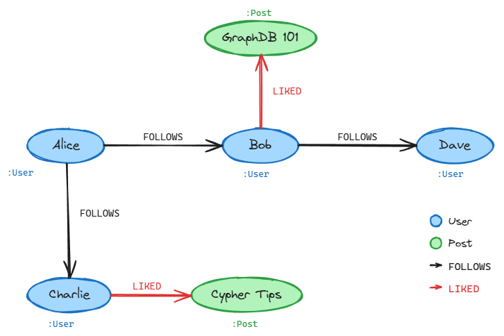
Consider a social network where users follow each other and like posts. To find all posts liked by Alice’s friends:

MATCH (alice:User {name: 'Alice'})-[:FOLLOWS]->(friend:User)-[:LIKED]->(post:Post)
RETURN friend.name, post.title

The MATCH clause describes a path pattern: start at a User node named Alice, traverse FOLLOWS edges to her friends, then traverse LIKED edges to reach Post nodes. In SQL, this would require joining three tables (users, follows, likes) with explicit foreign key conditions. In Cypher, the relationships are the query.

Where graph databases really shine is variable-depth traversal. To find all users reachable from Alice through up to 3 levels of FOLLOWS relationships:

MATCH (alice:User {name: 'Alice'})-[:FOLLOWS*1..3]->(connection:User)
RETURN DISTINCT connection.name

The *1..3 syntax tells the engine to follow FOLLOWS edges at any depth from 1 to 3 hops. In SQL, you would need a recursive CTE that self-joins the follows table up to three times, and performance degrades as the depth increases. Graph databases handle this natively because traversing edges is their fundamental operation, not an afterthought bolted onto row-based storage.

Spatial Database

Spatial databases are designed for storing and querying spatial data, such as map locations. They utilize spatial indexes to perform spatial queries efficiently, like finding all locations near a specific region. Common indexing mechanisms include quadtrees (which recursively subdivide 2D space into four quadrants), R-trees (which group nearby objects into bounding rectangles, excelling at range queries and nearest-neighbor searches), and geohashes (which encode latitude/longitude into a single string, enabling efficient prefix-based proximity lookups). The choice of index depends on the query patterns: quadtrees work well for uniformly distributed point data, R-trees excel with overlapping regions and polygons, and geohashes are simple to implement and integrate with key-value stores.

Quadtree

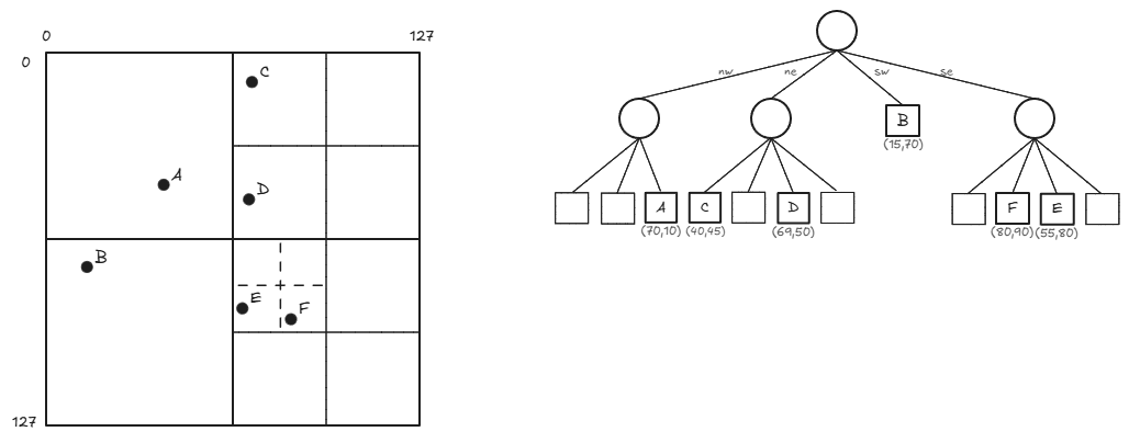
A quadtree is a tree data structure commonly used to index two-dimensional spatial data. Each node in a quadtree has either zero child nodes (leaf nodes) or exactly four child nodes. Quadtree nodes typically contain spatial data, such as map locations, with a maximum capacity of a specified number n.

As long as nodes are not at capacity, they remain leaf nodes; when they reach capacity, they are given four child nodes, and their data entries are distributed among the children. Quadtrees are well-suited for storing spatial data, as they can be represented as a grid filled with rectangles that are recursively subdivided into four sub-rectangles. Each quadtree node corresponds to a rectangle, and each rectangle represents a spatial region.

Querying Spatial Data

PostGIS, a spatial extension for PostgreSQL, is one of the most widely used tools for spatial queries. Here is a query that finds all coffee shops within 500 meters of a given point:

SELECT name, address
FROM coffee_shops
WHERE ST_DWithin(
    location::geography,
    ST_MakePoint(-73.9857, 40.7484)::geography,
    500
);

The ::geography cast tells PostGIS to treat coordinates as points on a spherical earth and compute distances in meters (without it, ::geometry operates in the coordinate system’s units, which for latitude/longitude would be degrees). Under the hood, PostGIS uses R-tree indexes built on GiST (Generalized Search Tree) to avoid scanning every row. The ST_DWithin function leverages this index to quickly narrow down candidates before computing exact distances, making proximity searches efficient even over millions of rows.

Choosing the Right Storage Paradigm

Paradigm	Use when	Not ideal for
Blob Storage	Large unstructured binary data (images, backups). Simple put/get by key	Queries that filter within content. ACID transactional workloads
Time Series DB	Time-stamped, append-mostly data (metrics, IoT, financial ticks). Time-windowed aggregations	Frequent updates or deletes. Complex entity relationships
Graph Database	Rich interconnected relationships with variable depth (social networks, fraud detection)	Simple tabular data. Write-heavy bulk ingestion
Spatial Database	Geographic or geometric data (maps, proximity search, route planning)	Non-spatial data. Workloads that never query by location

In practice, production systems often combine multiple paradigms. A ride-sharing application, for example, might use a relational database for user accounts and trip records, blob storage for driver documents and receipts, a spatial database for real-time proximity matching, and a TSDB for tracking ride metrics and surge pricing signals.

Related posts: SQL vs NoSQL Databases, Replication And Sharding