Big O Notation

You have an array of 10,000 users and need to find one by name. A linear search checks up to 10,000 entries. Binary search on a sorted array checks about 14. That difference, O(n) vs O(log n), is what Big O notation captures.

Both approaches solve the same problem, but one scales dramatically better than the other. Big O gives us a shared language to talk about that scaling behavior without getting bogged down in hardware specifics, programming languages, or constant factors that vary from machine to machine.

How Does the Work Grow?

The core question Big O answers is: as the input grows, how does the number of operations grow?

It does not tell you how many milliseconds something takes. It tells you the shape of the growth. If you double the input size, does the work double? Quadruple? Stay the same? That growth rate is what determines whether your solution works on a million records or falls apart.

Think of it this way. An O(n) algorithm that processes 1,000 items will need roughly 2,000 operations for 2,000 items. An O(n²) algorithm that handles 1,000 items comfortably will need four times the work for 2,000 items. At 10,000 items, it needs 100 times the work. The growth rate dominates everything else at scale.

Common Complexity Classes

Here are the most common Big O complexities, ordered from fastest to slowest growing:

• Constant: O(1) – the work stays the same regardless of input size
• Logarithmic: O(log n) – the work grows slowly, roughly halving the problem each step
• Linear: O(n) – the work grows proportionally to the input
• Log-linear: O(n log n) – typical of efficient sorting algorithms
• Quadratic: O(n²) – the work grows as the square of the input
• Factorial: O(n!) – the work grows astronomically fast

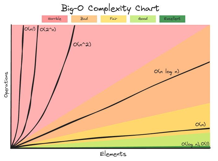
The graph makes the differences vivid. O(1) and O(log n) are practically flat compared to the explosive growth of O(n²) and beyond. This is exactly why choosing the right algorithm matters so much.

Code Examples for Each Complexity Class

O(1) – Constant Time

public static int getFirst(int[] array) {
    return array[0];
}

No matter whether the array has 10 elements or 10 million, accessing an element by index takes the same amount of time. The size of the input is irrelevant.

O(log n) – Logarithmic Time

public static int binarySearch(int[] sortedArray, int target) {
    int left = 0;
    int right = sortedArray.length - 1;

    while (left <= right) {
        int mid = left + (right - left) / 2;
        if (sortedArray[mid] == target) {
            return mid;
        } else if (sortedArray[mid] < target) {
            left = mid + 1;
        } else {
            right = mid - 1;
        }
    }
    return -1;
}

Each iteration cuts the search space in half. Doubling the input size adds only one extra step. For an array of 1,000,000 elements, binary search needs at most about 20 comparisons.

O(n) – Linear Time

public static int sum(int[] array) {
    int total = 0;
    for (int element : array) {
        total += element;
    }
    return total;
}

We visit every element exactly once. Double the array size and the work doubles. This is as good as it gets when you need to look at every element.

O(n²) – Quadratic Time

public static void printAllPairs(int[] array) {
    for (int i = 0; i < array.length; i++) {
        for (int j = 0; j < array.length; j++) {
            System.out.println(array[i] + ", " + array[j]);
        }
    }
}

For each element, we loop through every other element. An array of 100 produces 10,000 pairs. An array of 1,000 produces 1,000,000. You can see how this gets out of hand quickly.

Why Constants Don’t Matter

You might wonder why we write O(n) instead of O(2n) or O(5n). The reason is that Big O describes the growth rate, not the exact count of operations. Constants affect how fast something runs on a specific machine, but they do not change how it scales.

Consider two algorithms, one that does 2n operations and another that does 100n. Both are O(n). Yes, the second one is 50 times slower in practice, and that matters for performance tuning. But as n grows, both scale the same way: double the input, double the work. Compare either of them to an O(n²) algorithm, and at large enough inputs the quadratic one will always lose, even if its constant factor is tiny.

Here are the simplification rules:

Drop constants. O(25) becomes O(1). O(2n) becomes O(n). The constant does not change the shape of the growth curve.

Drop lower-order terms. O(n² + 2n) becomes O(n²). As n grows large, n² dominates completely. When n is 1,000, n² is 1,000,000 while 2n is just 2,000. The linear term becomes noise.

Another example: O(n! + n³ + log n + 3) simplifies to O(n!), because factorial growth dwarfs everything else.

Multiple Inputs Are Different

There is one important exception to dropping terms. When an algorithm operates on two separate inputs, you cannot simplify across them.

Consider a function that iterates over one array of size m and another of size n. Its complexity is O(m + n), and you cannot reduce it to O(m) or O(n). You can imagine a scenario where m is 2 and n is 1,000,000. Dropping either variable would hide meaningful information about how the algorithm behaves.

The same applies to O(m² + n). You can still drop constants (O(2m² + 3n) becomes O(m² + n)), but you must keep both variables because they represent independent inputs.

Amortized Complexity

Sometimes looking at the worst case of a single operation gives a misleading picture. A good example is Java’s ArrayList.

When you call add() on an ArrayList, the element is usually just placed into the next open slot in the backing array. That is O(1). But occasionally, the backing array is full. When that happens, ArrayList allocates a new array (typically 1.5 times the old capacity), copies everything over, and then inserts the new element. That single operation is O(n).

If you only looked at the worst case, you might conclude that ArrayList insertions are O(n). But that expensive copy happens less and less frequently as the array grows. After copying n elements into a new array, you get n more cheap insertions before the next resize. When you spread the cost of the occasional O(n) copy across all the O(1) appends, each insertion costs O(1) amortized.

This concept, amortized complexity, is the average cost per operation over a sequence of operations. It is a more honest description of how dynamic arrays actually perform in practice.

Big O vs Big Theta vs Big Omega

Big O is not the only asymptotic notation, though it is by far the most commonly used in practice.

• Big O (O) describes an upper bound. Saying an algorithm is O(n²) means the number of operations grows no faster than n² (up to a constant factor) for large inputs. It is a ceiling.
• Big Omega (Ω) describes a lower bound. Saying an algorithm is Ω(n) means it needs at least n operations.
• Big Theta (Θ) describes a tight bound, meaning the algorithm is both O(f(n)) and Ω(f(n)). A simple loop over an array is Θ(n): it is exactly linear.

In everyday engineering, we almost always say “Big O” and mean it as a tight bound. When someone says “this algorithm is O(n log n),” they typically mean it is also Θ(n log n), not just that it is bounded above by n log n. Technically imprecise, but universally understood.

Best, Average, and Worst Case

Big O usually refers to the worst-case scenario, but it is worth noting that some algorithms behave very differently depending on the input. QuickSort, for example, is O(n log n) on average but O(n²) in the worst case (when the pivot choices are consistently bad). Knowing which case you are analyzing matters, and when someone states a Big O without qualification, they almost always mean worst case.

Related posts: Complexity Analysis, Arrays, Logarithms in Algorithm Complexity